Transport with Capacities on a Line — Solution
Method and contribution
Use the problem setter's residual-transport model, ordered set of available storage sites, and sign-aware segment tree. Codex (GPT-6) supplies the optimality argument, explicit complexity bounds and standard C++17 implementation. A block-decomposition solution and program give a workload bound independent of sign changes. The segment-tree program is the preferred implementation.
Net flow and marginal cost
Let \(f_i\) be the net flow across edge \((i,i+1)\) , positive to the right. Opposite shipments can cancel, and the remaining flow decomposes into transports from production points to storage. Its minimum cost is
Adding one unit to the right changes the edge cost by
Adding one unit to the left decreases \(f_i\) : its marginal cost is \(-d_i\) for positive flow and \(d_i\) otherwise. A negative marginal cost cancels existing transport; it is not a negative physical distance.
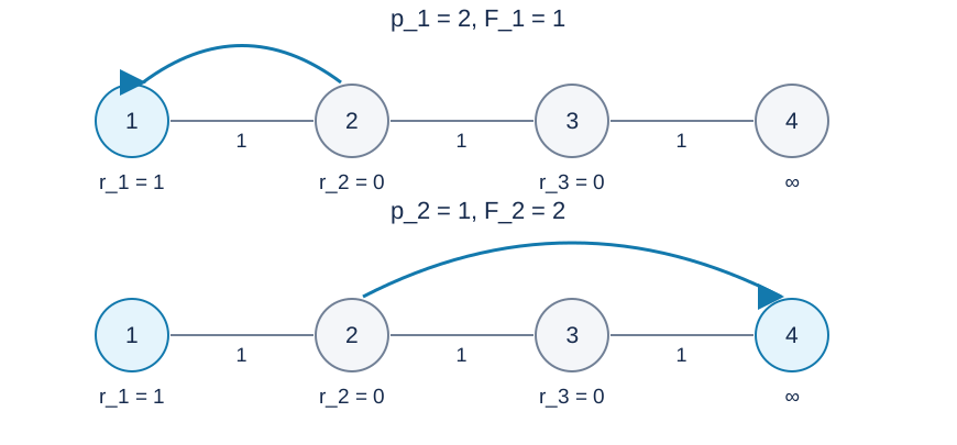
In the figure, \(r_1=1,r_2=r_3=0\) , all three distances are one, point four is the warehouse, and requests are \(2,1\) . The first item goes to point one at cost one. After the second request, move the first item to the warehouse and keep the new item at point one, giving total cost two. Fixing the first item's destination would miss this reassignment.
In the figure, \(F_j\) is the minimum cost for the first \(j\) items.
Why each augmentation is optimal
Represent roads by directed cost edges in both directions and storage capacity by edges to a sink. Keep an optimal flow for the previous prefix and supply one extra unit at the new production point. Residual edges can undo earlier transport, and the residual network of an optimal flow has no negative-cost cycle.
The difference between old and new feasible flows decomposes into an augmenting path to available storage and residual cycles of nonnegative cost. A cheapest augmenting path therefore gives a globally optimal assignment for the new prefix. Earlier items may change destinations, as allowed by the statement.
Only the closest site with space on each side needs consideration. A residual path from any available site \(L\) to a farther available site \(R\) cannot have negative cost. Otherwise, adding an item at \(L\) and using that path would make the enlarged problem cheaper than the old optimum. But deleting the new item's nonnegative-cost shipment from any enlarged solution gives a feasible old solution of no greater cost. The optimum cannot decrease when an item is added, a contradiction.
A route to a farther vacancy passes through the nearest one, and the remaining suffix has nonnegative cost. Stopping at the nearest vacancy is therefore no worse. If the production point itself has room, zero cost is already optimal.
Data structures
An ordered set stores sites with remaining capacity, always including the unlimited warehouse. If the origin is full, find the nearest vacancy on each side, compare the two marginal path costs, choose a minimum, shift the corresponding edge flows by one and consume a destination slot. Either side is valid on a tie: the next step only needs an optimal current flow.
Each segment-tree node stores total distances for negative, zero and positive flows; the greatest negative flow; the least positive flow; the number of zero-flow edges; and a lazy shift. A rightward query is zero plus positive minus negative distance sums. A leftward query is zero plus negative minus positive sums.
If a full-range unit shift changes no negative/zero/positive category, update only extrema and the lazy tag. Otherwise descend, reclassify leaves and combine statistics. Even zero-length edges may change flow category, so a zero distance sum cannot replace the zero-flow edge count.
A pending tag preserves every category. Thus child distance sums remain valid for queries without pushing the tag. A later partial update must push the actual flow change first.
Complexity and applicability
Let \(Z\) count all leaf transitions between negative, zero and positive flow categories. A full-range update that must descend contains such a transition; charge its extra descent to the affected leaf's ancestors. This gives \(O(n+(m+Z)\log n)\) total time and \(O(n)\) space. An update can visit the whole tree, so a safe general worst-case bound is \(O(nm)\) . Lazy tags alone do not establish logarithmic time per update.
The block program has an explicit bound on scans and sorting for every operation; see its separate explanation. Both programs pass the formal recipes at the original limits; see the measurements. The segment tree is faster on those inputs, while the time limit also gives the block program twofold headroom. A finite stress set does not prove a stronger amortized segment-tree bound.
One path cost is bounded by the total line length, about 1.2 million here. The total is at most \(m\sum_i d_i\) , so use 64-bit arithmetic. Zero capacities, zero distances, repeated origins and complete overflow into the warehouse require no different model.
Data and reproduction
The statement contains three samples. The test plan defines ten scored inputs. The generator uses only the Python standard library and accepts --plan, --out-dir, --case and --std. Large generated inputs and executables are kept outside the published package. See the reference measurements for runtime and memory.