A Common Connected Set in Several Trees: Solution
Problem setter’s solution: centroid decomposition of the first tree, with maximum-weight closure for sets containing the decomposition vertex. GPT-6 adds the pruning/min-cut proofs, 64-bit capacities, and explicit traversal stacks.
1. Classify sets by a decomposition vertex
Choose a centroid \(c\) of the current component \(U\) in the first tree. A nonempty feasible set either contains \(c\) , in which case this level handles it, or avoids \(c\) . In the latter case, connectivity in the first tree places the entire set in one component left after removing \(c\) .
Solve the current level, remove \(c\) , and process those components. The answer is the maximum over all levels and zero. Centroids give \(O(\log n)\) decomposition depth.
2. Remove vertices that cannot coexist with the root
Restricting another tree to \(U\) may disconnect it. In each tree, traverse from \(c\) using only vertices in \(U\) , recording reached vertices and their parents.
A vertex unreachable in any tree cannot belong to a feasible set containing \(c\) , so delete it. Propagate deletions: if a vertex is deleted, its descendants in any of the rooted trees must also be deleted. A queue follows the recorded parent-child edges until no new deletion occurs.
The remaining set \(V\) contains the complete ancestor chain to \(c\) in every tree, so it is connected in every tree. Conversely, no feasible set containing \(c\) loses a vertex: the initial deletions are necessary, and every propagated deletion follows from a missing required ancestor. The pruning is therefore both safe and sufficient.
3. Maximum-weight closure
For every non-root vertex \(u\) in \(V\) , add a directed constraint from \(u\) to its parent in each tree. Selecting \(u\) requires selecting every destination. This is a closure constraint. Every nonempty closed set contains \(c\) through its ancestor chains; the empty set remains allowed.
Let \(P=\sum_{u\in V}\max(a_u,0)\) . Build a flow network:
- For \(a_u>0\) , add source-to-\(u\) capacity \(a_u\) .
- For \(a_u<0\) , add \(u\)-to-sink capacity \(-a_u\) .
- Give every closure edge capacity \(P+1\) .
The empty selection gives a cut of capacity \(P\) , so a minimum cut never cuts a closure edge. If its selected source-side set is \(S\) , the cut capacity is
The answer for this level is exactly \(P-\operatorname{maxflow}\) . Do not force \(c\) onto the source side: every nonempty closure already contains it, while an all-negative instance may choose nothing.
If \(P\) does not exceed the current answer, skip this flow computation, since no selection at the level can exceed \(P\) .
4. Implementation and correctness
Centroid traversals, rooted-tree traversals, deletion propagation, and Dinic blocking flow use explicit queues or stacks. A blocking-flow frame stores its vertex, flow limit, amount already sent, and incoming edge. Returning from a child updates forward and reverse residual capacities by the same amount. This avoids call-stack failure on long paths.
Use 64-bit integers for every capacity and returned flow. The positive sum may reach \(20000\cdot10^9\) , so total source flow and total reward require 64-bit storage. The finite value \(P+1\) already supplies sufficient infinity.
Pruning preserves every eligible set at a level; minimum cut finds its optimum exactly; decomposition assigns every remaining feasible set to a later component. Taking the maximum therefore gives the global optimum.
5. Complexity and scope
Each vertex appears in \(O(\log n)\) components. Even when another tree contains high-degree vertices, charging adjacency scans to each vertex’s appearances bounds graph preparation by \(O(mn\log n)\) .
A component of size \(s\) yields \(O(s)\) network vertices and \(O(ms)\) edges. Generic Dinic gives a conservative \(O(ms^3)\) bound. Geometrically shrinking centroid components sum to a conservative \(O(mn^3)\) flow bound, in addition to graph preparation. Flow computation is not claimed to take logarithmic time. Practical performance depends on network structure and requires full-range measurements and target-environment calibration.
Space is \(O(mn)\) , retaining only the current network. For one tree, a maximum-connected-subtree DP also works, but it does not directly enforce multiple-tree constraints and is not a second full-range solution.
Illustration
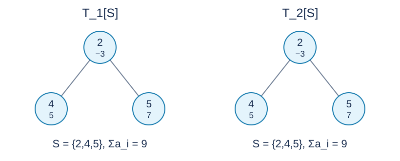
The figure shows only the two induced subgraphs \(T_1[S],T_2[S]\) on the selected set \(S=\{2,4,5\}\) in sample two. Each circle shows its ID above its weight. Both subgraphs are connected and their total weight is nine.
Data and reproduction
The statement contains three samples. The test plan defines ten scored inputs. The generator uses only the Python standard library and accepts --plan, --out-dir, --case and --std. Large generated inputs and executables stay outside the published package. See the reference measurements for runtime and memory.