Edit Town and Simoleons: Solution¶

Algorithm and Attribution¶

Codex (GPT-6) provides the optimality proof for sorted averaging, all seven statistics, and an exact backward threshold comparison. std.cpp uses the stated single-person target and initial household-size limit of 20.

Individual Wealth¶

Splitting a household into single-person households gives each resident its initial per-capita wealth. Merging a group and splitting it again replaces their individual values by their mean. Each permitted move also has this averaging interpretation, so analyze the vector of individual wealths.

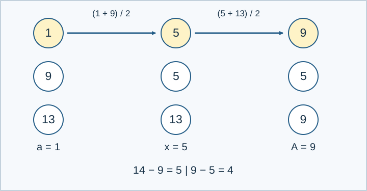
Let the target initially hold \(a=m_1\) . Use only outsiders initially holding \(v>a\) , in nondecreasing order of \(v\) . Merge each with the target into a two-person household and split them again. The target changes from \(x\) to \((x+v)/2\) . Use each outsider at most once.

Two averages in increasing wealth order

Optimality Under Arbitrary Editing¶

For any current wealth vector, define \(\Phi\) as the result of this sorted strategy. It is the maximum over all sequential averaging plans that use each outsider at most once. For adjacent values \(u\le v\) , using \(u\) then \(v\) gives \((v-u)/4\) more than the reverse order; subsequent averages preserve the sign. Thus sorting is optimal. After sorting, values no larger than the starting target can be deleted, while every omitted richer value can be inserted in order to increase the result.

Any two-person average cannot increase \(\Phi\) :

Neither person is the target: \(\Phi\) is the maximum of linear functions corresponding to distinct-person sequences, hence is convex in outsider values. It is also symmetric under outsider permutations. Averaging two coordinates averages a vector and its swapped copy, so convexity proves nonincrease.
The target averages with someone richer: that outsider then equals the new target and is not reused by the subsequent sorted strategy. The combined procedure is still a distinct-person sequence from the previous state, bounded by its \(\Phi\) .
The target averages with someone no richer: the target decreases, and the other person equals it and is not reused. With that outsider removed, \(\Phi\) is monotone in the starting target wealth, again proving nonincrease.

A group average is the limit of cyclic pair averages within that group: squared deviations decrease and converge to zero. As a maximum of finitely many linear functions, \(\Phi\) is continuous. It therefore cannot increase under group averages either. Initial \(\Phi\) bounds every allowed editing process, and the sorted strategy attains it in finitely many steps, proving the optimum \(A\) .

Process Whole Initial Households¶

The \(p\) residents of one initial household share the value \(v=m/p\) . Processing all of them changes the target to

\[ x'=v+(x-v)2^{-p}. \]

Sort ratios \(m/p\) using cross multiplication. Each household requires one modular update; precompute inverses of 1 through 20 and \(2^{-p}\) . Skip households with \(v\le a\) . In sorted order the target stays below the next richer value, so every used outsider strictly increases it.

Minimum Outsider Wealth and the Per-Capita Gap¶

Let \(Q\) be the number of outsiders and \(O=\sum_i m_i-A\) their final total wealth. Handle \(Q=0\) directly. Otherwise let \(v_{\min}\) be their minimum initial per-capita wealth. The smallest possible outsider individual wealth at the optimum is

\[ b=\begin{cases}v_{\min},&v_{\min}\le a,\\(a+v_{\min})/2,&v_{\min}>a.\end{cases} \]

In the first case, averaging cannot decrease the global minimum, and the strategy leaves such a person untouched. In the second, the first effective group average involving the target includes outsiders worth at least \(v_{\min}\) . Its result is at least \((a+v_{\min})/2\) , after which no individual can fall below this value. The first step of the sorted strategy attains it.

In any optimal arrangement, no outsider household can have per-capita wealth above \(A\) : splitting out one such person and averaging them with the target would improve the optimum. Hence the maximum per-capita gap is \(A-b\) , attained by isolating the poorest outsider after the sorted strategy.

Household Wealth Gap¶

For \(Q=1\) , the only arrangement consists of two single-person households, giving \(|A-O|\) . For \(Q\ge2\) ,

\[ G=\max(A-b,\ O-2b,\ O-A). \]

If the target is richest, the gap is at most \(A-b\) . If it is poorest, an outsider household holds at most \(O\) . If both extremes are outsiders, the poorest holds at least \(b\) and the richest at most \(O-b\) . Isolating the poorest outsider and grouping the remaining outsiders realizes lower bounds for the first two candidates. Grouping all outsiders realizes the third. Thus their maximum is attainable.

If any outsider was initially richer, the last used outsider finishes with wealth \(A\) too. For \(Q\ge2\) , this implies \(O\ge A+b\) and simplifies the gap to

\[ G=O-\min(A,2b). \]

If nobody was richer, \(A=a\) is an integer. Compare the three candidates after multiplying by the denominator of \(v_{\min}\) .

Four Predicates¶

After the sorted strategy every outsider individual holds at most \(A\) . Splitting everyone proves that predicates 4 and 6 are always true.

Because the target has one resident, both strict predicates are equivalent to \(AQ>O\) . Necessity follows from totals: if each outsider household has total wealth below \(A\) , its per-capita wealth is also below \(A\) , so their overall mean is below \(A\) . For sufficiency, merge all outsiders and split them into single-person households, each holding \(O/Q<A\) .

No huge rational comparison is needed. With a richer outsider, \(Q=1\) ends in a tie; for \(Q\ge2\) at least one person besides the last used outsider is strictly poorer, so both strict predicates are true. With no richer outsider, they hold exactly when some outsider was initially strictly poorer.

Compare \(A\) and \(2b\) Exactly¶

Residues do not preserve order, and floating-point arithmetic can round an extremely small difference to zero. Use the scale

\[ D=2\operatorname{lcm}(1,2,\ldots,20)=465585120. \]

Every initial per-capita value and \(b\) become integers after multiplication by \(D\) . The optimum \(A\) may still have a huge binary denominator. Instead of constructing it, propagate the required threshold backward.

For threshold \(T\) and a batch of \(p\) richer people with scaled wealth \(V\) ,

\[ x'=V+(x-V)2^{-p}\ge T\quad\Longleftrightarrow\quad x\ge V+2^p(T-V). \]

Start with \(T=2bD\) and process richer households in reverse order:

If \(T\le aD\) , the condition is certainly true.
If \(T\ge V\) , it is false because the target after this batch is strictly below \(V\) .
Otherwise set \(\delta=V-T>0\) . If \(2^p\delta>V-aD\) , the preceding threshold is below the initial wealth, so return true. First compare \(\delta>\lfloor(V-aD)/2^p\rfloor\) to avoid overflow.
Otherwise safely replace the threshold by \(V-2^p\delta\) and continue.

All thresholds remain bounded integers and every step preserves the condition, including exact equality. Scaled initial wealth is below \(4.66\times10^{14}\) . When nobody is richer, the common-denominator gap numerators are at most \(2\times10^{13}\) . Both fit signed 64-bit integers. Modular products also fit because both factors are below \(P\) .

Complexity and Validation¶

Time is \(O(n\log n)\) and space is \(O(n)\) , independent of expanded population. The required extrema use only initial population denominators and powers of two, so their modular inverses exist. No such claim is needed for every possible intermediate editing state.

Independent checks include arbitrary subset averages against the potential, exhaustive outsider partitions, expanded-population Fraction arithmetic, and backward histogram contributions. Formal cases include differences too small for ordinary floating-point arithmetic. See tests and performance.