GitHub 源文件 Markdown 中文

Nomadism — Day — Solution

Comparing solutions

A tour in input-index order, returning to the start, ignores the coordinates. This produces a tour but cannot guarantee its length. For points \((0,0),(100,0),(1,0),(101,0)\) in that order, the tour has length \(400\) , while the MST weighs \(101\) . The permitted bound is only \(2.001\times101+0.001=202.102\) .

The implementation used by Codex (GPT-6) doubles an Euclidean MST traversal and shortcuts by the triangle inequality, using Delaunay candidate edges to avoid the complete graph. It takes \(O(n\log(n+1))\) time and \(O(n)\) space; the proof and degeneracies are covered below. Geometric construction adds work but provides the required guarantee. Linear-time index output is not a valid competing algorithm for this task.

Constructing a tour from a minimum spanning tree

Use farms as vertices and the prescribed distance as the weight of each undirected edge. The minimum connection cost \(M\) is the weight of a minimum spanning tree (MST) of this complete graph: deleting cycle edges from any connected graph leaves a spanning tree without increasing its weight.

Compute an MST \(T\) , root it at farm \(1\) , and traverse it in depth-first order. Append each vertex when it is first visited, then append \(1\) again at the end. The implementation uses an explicit stack so that a long path cannot overflow the call stack.

Why the cost is at most twice the tree weight

A full walk along the tree, returning along every edge, traverses each edge twice and costs exactly \(2M\) . Remove repeat visits from this walk, keeping the first occurrence of each vertex and the final return to the start. By the triangle inequality, replacing a path segment by a direct edge never increases its cost. The resulting tour therefore satisfies:

\[ C\le2M \]

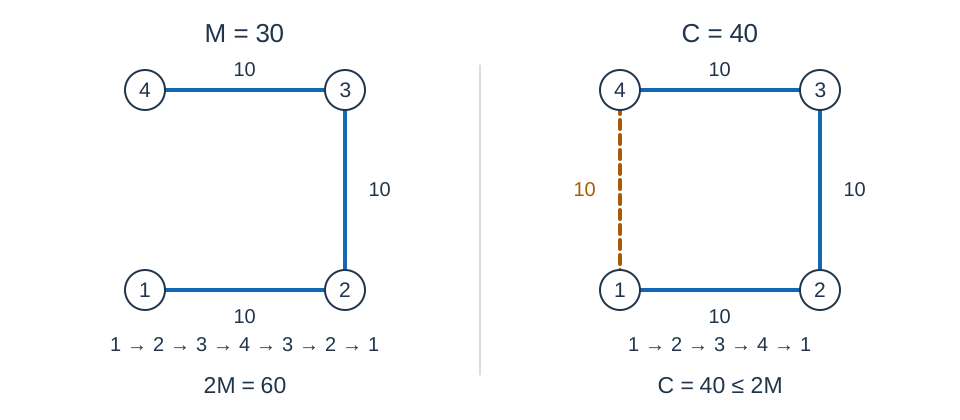
The full walk on the left is \(1,2,3,4,3,2,1\) and costs \(60\) . Skipping repeated visits produces the tour \(1,2,3,4,1\) on the right, costing \(40\) .

If the shortest tour has length \(OPT\) , removing one edge from it leaves a spanning tree, so \(M\le OPT\) . The reference construction satisfies \(C\le2OPT\) . The judging tolerance permits \(C\le2.001M+0.001\) , so not every accepted tour is necessarily a strict 2-approximation.

Coincident points and boundary cases

Sort farms by coordinates and keep one representative of each distinct position. Join every other farm at that position to its representative by a zero-weight edge. Compute a tree only on the distinct positions, then include these zero-weight edges. This preserves \(M\) and ensures that every original farm number appears in the tour.

For a single farm, print 1 1 . If all farms coincide, \(M=C=0\) . General position is not assumed, and no random perturbation changes coordinates or weights.

Does rounding up preserve the MST?

Every MST under true Euclidean distance remains an MST after rounding each edge weight up separately. We may therefore use Euclidean geometry to select candidate edges, run Kruskal in squared-distance order, and sum the rounded lengths of the selected edges. There are two properties to verify: one for shortcutting the tour, and one for finding the tree.

1. The triangle inequality survives

Let \(e(a,b)\) be true Euclidean distance and \(d(a,b)=\lceil e(a,b)\rceil\) the required edge weight. Euclidean distance obeys the triangle inequality, and \(\lceil u+v\rceil\le\lceil u\rceil+\lceil v\rceil\) . Thus:

\[ d(a,c)\le\lceil e(a,b)+e(b,c)\rceil\le d(a,b)+d(b,c) \]

The earlier proof that shortcuts cannot increase the tour cost therefore applies to this task. Rounding down would not necessarily preserve this property.

2. A complete cut-and-exchange proof for the MST

Let \(T\) be an MST for true distance, and let \(f\) be any nondecreasing function: \(x\le y\) implies \(f(x)\le f(y)\) . Here \(f(x)=\lceil x\rceil\) .

Delete any tree edge \(e\) from \(T\) . This splits the tree into two components \(A,B\) . Such a partition is called a cut, and an edge with one endpoint on each side crosses that cut. For every crossing edge \(g\) :

\[ w(e)\le w(g)\quad\Longrightarrow\quad f(w(e))\le f(w(g)) \]

Otherwise, replacing \(e\) with \(g\) would make the original tree cheaper, contradicting its optimality.

We must also show why these comparisons guarantee a minimum total after transformation. Take any other spanning tree \(S\) . If \(S\ne T\) :

1. Choose an edge \(e\) in \(T\) but not in \(S\) , and consider the cut \(A,B\) above.
2. The unique path in \(S\) between the endpoints of \(e\) must cross that cut. Choose a crossing edge \(g\) on this path.
3. The edge \(g\) is not in \(T\) : the only edge of \(T\) crossing this particular cut is \(e\) , which is absent from \(S\) .
4. Add \(e\) to \(S\) and remove \(g\) from the resulting cycle. The result is still a spanning tree. Its total transformed weight does not increase, and it contains one more edge of \(T\) .

After at most \(n-1\) exchanges, \(S\) has become \(T\) without any increase in transformed weight. Since \(S\) was arbitrary, \(T\) is also optimal under the new weights. Equal weights are allowed throughout, so ties introduced by rounding cause no problem.

Kruskal gives another way to understand this: an ordering by true distance remains a valid nondecreasing ordering after rounding up. Using that same order and the same disjoint-set operations chooses the same MST. Squared distance has the same ordering as true distance, so edge sorting needs no square roots.

3. What this result does and does not assert

Rounding can introduce additional optimal trees. For \(A=(0,0),B=(5,0),C=(2,4)\) , the three edge lengths are \(5,5,\sqrt{20}\) . A Euclidean MST must contain \(AC\) . After rounding, all three weights are \(5\) , so any two edges form an MST of weight \(10\) . We only need the candidate graph to retain an original Euclidean MST; it need not retain every tree that becomes optimal after rounding.

The proof relies on exchanging edges in a tree. It is not a claim that a monotone function preserves comparisons between arbitrary sums. The actual cost is:

\[ M=\sum_{e\in T}\lceil w(e)\rceil \]

This generally differs from \(\left\lceil\sum_{e\in T}w(e)\right\rceil\) . The implementation must round each selected edge separately.

Why use a triangulation?

The complete graph has \(n(n-1)/2\) edges, too many to generate for large inputs. We want a graph with only \(O(n)\) edges that still contains a Euclidean MST. The following sections build this graph from basic geometric concepts; only spanning trees and Kruskal are assumed as prerequisites.

1. Convex hulls and triangulations

Imagine stretching a rubber band around all the points and letting it tighten. Its boundary is the convex hull. When the points are not all collinear, the hull encloses a convex polygon.

A triangulation joins selected pairs of points to tile the interior of the convex hull with triangles, subject to these rules:

• Every input point is a vertex of the triangulation.
• Edges meet only at shared endpoints. They cannot cross or pass through another vertex.
• Triangle interiors do not overlap, and no input point is left inside a triangle.

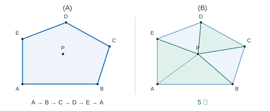
The point \(P\) lies inside the hull. The right panel incorporates it into the triangulation. The same points usually admit many triangulations. We need an additional condition to choose one suitable for finding an MST.

2. Delaunay triangulations and empty circles

Three noncollinear points determine a unique circle through them, called their triangle's circumcircle. A triangulation is a Delaunay triangulation if no triangle's circumcircle contains another input point strictly inside. Other sites may lie on the circle, so four cocircular points can lead to multiple valid answers. CGAL's triangulation guide uses this definition.

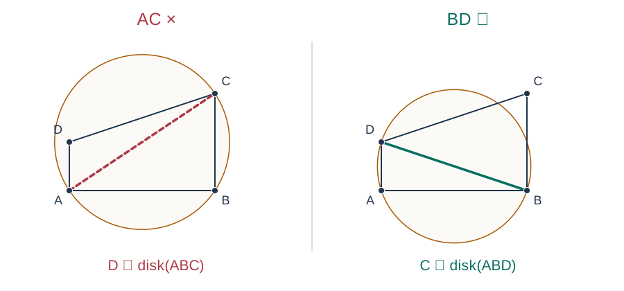
Here \(A=(0,0),B=(6,0),C=(6,4),D=(0,2)\) . The left triangulation uses \(AC\) , but \(D\) lies inside the circumcircle of \(\triangle ABC\) , so it is invalid. With \(BD\) instead, neither triangle's circumcircle contains the fourth point. Only the circumcircle of \(\triangle ABD\) is drawn on the right to keep the picture readable.

Replacing one diagonal of a quadrilateral with the other is called an edge flip. The divide-and-conquer algorithm does not first build an arbitrary triangulation and flip its edges one by one, but it uses the same in-circle test to decide which edges to remove and add.

3. How this relates to a Voronoi diagram

A Voronoi diagram partitions the plane into regions. A site's region consists of positions no farther from that site than from any other. If two regions share a boundary segment, join their sites to obtain a Delaunay edge. Polygonal faces caused by cocircular sites can be filled with diagonals to obtain a triangulation.

Thus, using a Voronoi diagram to find a Euclidean MST is a valid approach. The reference program directly builds the corresponding Delaunay triangulation, avoiding coordinates of Voronoi vertices, circumcenters, and boundary intersections.

4. Why a Euclidean MST is retained

Take an edge \(AB\) of a Euclidean MST and consider the closed disk with diameter \(AB\) . If it contains another distinct site \(P\) , then:

\[ |AP|<|AB|,\qquad |BP|<|AB| \]

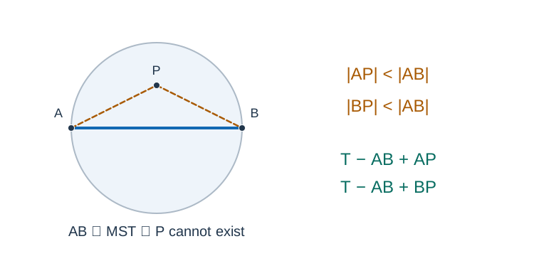
Removing \(AB\) from the tree puts \(P\) in either the component of \(A\) or that of \(B\) . In the former case, reconnect with the shorter edge \(PB\) ; in the latter, use \(PA\) . Either choice contradicts optimality. Thus the disk, including its boundary, contains no input sites except \(A,B\) .

At the center of that disk, \(A,B\) are equally close and strictly closer than every other site. Move a sufficiently small distance along the perpendicular bisector of \(AB\) : this strict comparison still holds. The two Voronoi regions therefore share a boundary segment, and the corresponding edge \(AB\) must be in the Delaunay triangulation. This also removes any concern about optional diagonals for cocircular sites: the MST edges we need are mandatory edges. CGAL's Euclidean MST example follows exactly the approach of building a Delaunay triangulation and running Kruskal.

Consequently, building the Delaunay graph for true distance, finding a Euclidean MST, and rounding its edge lengths individually gives the exact \(M\) required here. If all sites are collinear, keeping consecutive edges in position order is sufficient instead.

5. Why the number of edges is linear

Suppose there are \(k\) distinct sites and they are not all collinear. Let \(E\) be the number of edges and \(F\) the number of faces, including the unbounded outside face. Euler's formula for a plane graph gives \(k-E+F=2\) . Each face has at least three boundary edges, and each edge is counted by two faces, so \(3F\le2E\) . Together these give \(E\le3k-6\) . With all sites collinear, the chain has \(k-1\) edges.

The triangulation therefore reduces the number of candidate edges from quadratic to linear. The next task is to find those edges in \(O(k\log k)\) time.

Divide-and-conquer Delaunay: the overall structure

The reference program uses the Guibas–Stolfi divide-and-conquer algorithm, with \(O(k\log k)\) worst-case time. The original algorithm appears in Section 9 of the paper; Section 8 covers geometric predicates. The explanation below follows this task's implementation.

1. Sort distinct sites lexicographically by \((x,y)\) , once at the start.
2. Split a contiguous index range into a left half \(L\) and a right half \(R\) , and recursively triangulate both.
3. Merge by deleting old edges that are no longer suitable and adding cross edges, which join the two halves.
4. Return the merged triangulation and handles for edges at its leftmost and rightmost hull vertices, ready for the parent merge.

For two sites, add their edge. For three noncollinear sites, form a triangle; for three collinear sites, form a chain in position order. A single distinct site is handled before entering the recursion. Splitting four or more sites always leaves at least two in each half.

Equal horizontal coordinates are ordered by vertical coordinate. To understand the left/right separation in this case, imagine rotating the coordinate axes by a sufficiently small angle so that the new horizontal ordering equals the original lexicographic ordering. This changes only the viewing direction and preserves distances, collinearity, and cocircularity. The program still computes with the original integer coordinates; it does not rotate or perturb the points.

The main operation: merging two triangulations

1. Start at the lower common tangent

The lower common tangent connects the two convex hulls with every site above or on its line. Its endpoints give the first cross edge. Start at the rightmost vertex of the left hull and the leftmost vertex of the right hull, then move endpoints along their hulls until the line supports both hulls. Each endpoint advances along its hull; there is no need to enumerate all pairs.

Write the current endpoints as \(\ell\in L,r\in R\) . This explanation uses the direction \(\ell\to r\) , from left to right; the code stores Base in the opposite direction, \(r\to\ell\) . A point being “above” the current edge means it is to the left of the directed line \(\ell\to r\) , not merely that it has a greater vertical coordinate.

2. Why only one endpoint changes at a time

Imagine a vertical line separating \(L\) from \(R\) . All cross edges of the final triangulation intersect it and can be ordered by their intersections from bottom to top. Two consecutive cross edges border the same triangular face, so they share an endpoint.

Starting from \(\ell r\) , the next cross edge therefore has one of two forms:

• Keep the right endpoint \(r\) , move the left endpoint to some \(p\in L\) , and add \(pr\) .
• Keep the left endpoint \(\ell\) , move the right endpoint to some \(s\in R\) , and add \(\ell s\) .

Each step determines another triangle and advances through the region between the halves, eventually reaching the upper common tangent. This concrete example shows the complete merge.

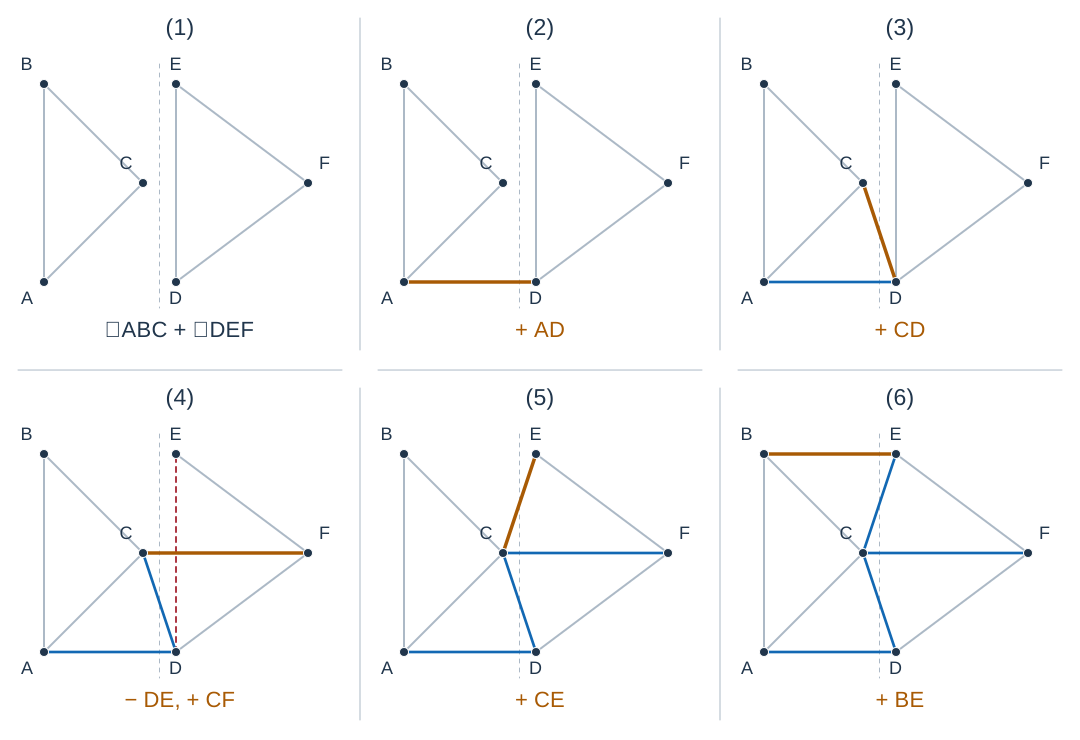
The coordinates are \(A=(0,0),B=(0,6),C=(3,3),D=(4,0),E=(4,6),F=(8,3)\) . The left half contains \(A,B,C\) , and the right half contains \(D,E,F\) . Dashed lines separate the halves; gray edges come from recursion, blue edges are earlier cross edges, and orange marks the current edge. Read left to right, then top to bottom: start at the lower tangent \(AD\) , move the left endpoint to \(C\) , the right endpoint to \(F\) and then \(E\) , and finally the left endpoint to \(B\) , reaching the upper tangent \(BE\) .

3. Find candidates and remove unsuitable old edges

On the left, start from direction \(\ell\to r\) and take the first adjacent edge \(\ell p\) counterclockwise around \(\ell\) . On the right, start from \(r\to\ell\) and take the first adjacent edge \(rs\) clockwise around \(r\) . A candidate must lie strictly above the current edge. Neighbors are ordered around the vertex in the plane, not by identifier, horizontal coordinate, or distance.

First clean the left side. Let \(\ell q\) be the next counterclockwise edge after \(\ell p\) . If \(q\) is strictly inside the circumcircle of \(\triangle\ell rp\) , then \(p\) is not yet the correct candidate. Delete the old edge \(\ell p\) , advance to \(q\) , and test its next neighbor. The right side is symmetric: if \(rt\) is the next clockwise edge after \(rs\) , and \(t\) is strictly inside the circumcircle of \(\triangle\ell rs\) , delete \(rs\) and continue with \(t\) .

These deleted edges came from a recursive result. An edge can be valid for one half in isolation but lose its empty-circle property when the other half is added. Simply adding cross edges while keeping every old edge would be incorrect.

If the next neighbor has wrapped below the current edge, cleanup also stops. As the disk expands above the edge, its lower part shrinks; the preceding empty circle ensures that lower sites cannot enter it. A repeated endpoint makes the in-circle determinant zero and cannot trigger deletion either.

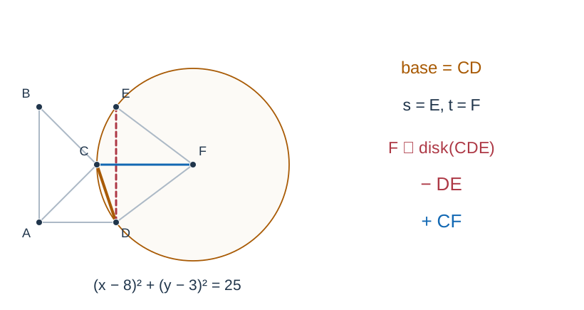
In the six-site example, the first right candidate at base \(CD\) is reached by \(DE\) . The circumcircle of \(\triangle CDE\) is \((x-8)^2+(y-3)^2=25\) . Since \(F=(8,3)\) is its center, \(DE\) must be removed. The right candidate then becomes \(F\) . Candidate cleanup is necessary for correctness.

4. Choose between the cleaned candidates

After cleanup, let \(p\) be the left candidate and \(s\) the right candidate:

• If neither side has a candidate above the current edge, it is the upper common tangent. Stop.
• If exactly one side has a candidate, choose that side.
• If both have candidates, test whether \(s\) lies strictly inside the circumcircle of \(\triangle\ell rp\) . If so, choose \(s\) and add \(\ell s\) . Otherwise, choose \(p\) and add \(pr\) .

For intuition, keep a circle passing through the fixed endpoints \(\ell,r\) and move its center along their perpendicular bisector. Expand the part of its disk above the current edge. The first new site touched determines the next triangle. If \(s\) is already inside the circle through \(p\) , it would have been touched earlier, so choose \(s\) . This describes the geometry; the code does not compute or move a circle center.

If four sites are cocircular, either choice satisfies the empty-circle condition. The implementation tests strictly for interior points. Equality does not trigger deletion, and the final choice between tied candidates favors the left one.

The six-site example can be checked step by step:

Current edge	Cleaned left and right candidates	Decision	New cross edge
\(AD\)	\(C,E\)	\(E\) is outside the circle of \(\triangle ADC\) ; choose left	\(CD\)
\(CD\)	No valid left candidate; \(F\) on the right	After deleting \(DE\) , only the right side is valid	\(CF\)
\(CF\)	\(B,E\)	\(E\) is inside the circle of \(\triangle CFB\) ; choose right	\(CE\)
\(CE\)	\(B\) ; no valid right candidate	Choose left	\(BE\)
\(BE\)	Neither side has a valid candidate	Upper common tangent reached	Stop

In particular, \(B\) has a greater vertical coordinate but lies to the right of the directed line \(C\to D\) . It is not a valid left candidate at base \(CD\) . Use the cross product for this decision.

5. Why testing neighboring candidates is enough

For an arbitrary graph, one outside neighbor would not justify stopping the search. The argument depends on both halves already being Delaunay triangulations.

Consider the left side. Translate and rotate the current edge so that \(\ell=(0,0),r=(a,0)\) , where \(a>0\) . An upper candidate \(p=(x,y)\) has \(y>0\) . The circle through \(\ell,r,p\) has center \((a/2,h(p))\) , with:

\[ h(p)=\frac{x^2+y^2-ax}{2y} \]

A higher center means that the disk covers more of the half-plane above the edge. Thus the first candidate touched is the one minimizing \(h(p)\) . The in-circle test compares these heights without actually computing a division.

Order the upper neighbors of \(\ell\) counterclockwise as \(p_1,p_2,\ldots\) . For Delaunay neighbors, the sequence \(h(p_i)\) decreases, may tie at its minimum, and then increases; either the decreasing or increasing part may be empty. Starting at the first neighbor and stopping at the first nondecreasing step therefore finds a minimum.

Start with neighbors in that side's original triangulation. Merging only removes some of these same-side edges, and taking a subsequence preserves the property above.

This property follows from the empty circles of adjacent triangles. Let \(b_i\) be the horizontal coordinate where the circumcircle of \(\triangle\ell p_i p_{i+1}\) meets the horizontal axis again, besides \(\ell\) ; set it to zero in the tangent case. Adjacent circles share \(\ell,p_{i+1}\) , and the next neighbor cannot lie inside the preceding circle. Along the ordered neighbors, these second intersections can therefore only move left. Comparing circle equations gives:

\[ h(p_{i+1})-h(p_i)=\frac{b_i-a}{2}\left(\frac{x_{i+1}}{y_{i+1}}-\frac{x_i}{y_i}\right) \]

The term in parentheses is strictly negative because the direction angle is increasing. Heights decrease while \(b_i>a\) ; once \(b_i\le a\) , they cannot decrease again. The right side follows by reflection. This is why the cleanup loop can stop at its first failed in-circle test instead of scanning all remaining sites.

Why is the first site touched among these neighbors at all? Its circle through \(\ell,r\) has not previously met any other site on that side. It therefore supplies an empty-circle witness on that side, making the segment to \(\ell\) a Delaunay neighbor edge. When several sites are cocircular, take the first tied site in the order around the vertex.

6. Merge correctness and pseudocode

At the lower common tangent, there is a circle through the current endpoints with no sites inside. Candidate cleanup finds the first site this circle would touch on each side. One further comparison finds the first site across both halves, producing a triangle whose circumcircle is empty for the entire input. Its new cross edge also has an empty-circle witness, so it can become the next base.

The discarded edges are not needed: the points on opposite sides of such an edge already create an in-circle conflict, preventing that edge from having an empty circle in the combined point set. Cross edges advance in their order along the separating line and do not cross the completed part. At the upper common tangent, the region between the two halves is filled, and the resulting triangulation satisfies the empty-circle condition.

This pseudocode uses the left-to-right endpoint convention of the explanation. Both next_ccw and next_cw navigate around the same origin; the next section explains how to support them.

Merge(L, R):
    (l, r) = lower_common_tangent(L, R)
    add edge l-r
    loop:
        lp = first edge counterclockwise from l->r
        if endpoint p is above l->r:
            while next endpoint q is inside circle(l, r, p):
                next = next_ccw(lp)
                delete lp
                lp = next

        rs = first edge clockwise from r->l
        if endpoint s is above l->r:
            while next endpoint t is inside circle(l, r, s):
                next = next_cw(rs)
                delete rs
                rs = next

        recompute whether p and s are above l->r
        if neither is valid: break
        if p is invalid or (s is valid and s is inside circle(l, r, p)):
            add edge l-s
            r = s
        else:
            add edge p-r
            l = p

Maintaining the edges with quad-edge

1. What an ordinary adjacency list lacks

An adjacency list finds all edges incident to a vertex. Merging needs constant-time access to the next edge around that vertex and the next edge along a face. Repeatedly sorting by angle, or searching and deleting in a linear container, could destroy the linear merge bound.

A quad-edge structure uses four records per undirected edge to encode both orders. Initially, think of it as a collection of editable circular lists. Geometric computations still use only the original sites.

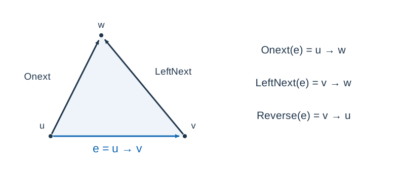
The triangle \(u,v,w\) is counterclockwise. Onext(e) advances counterclockwise around origin \(u\) . LeftNext(e) continues along the boundary of the face to the left of \(e\) , starting at \(v\) . These are different notions of the next edge.

2. Four records and the navigation functions

In mst.hpp, undirected edge \(j\) occupies indices \(4j,4j+1,4j+2,4j+3\) . Offsets \(0,2\) represent the two directions of the original edge. Offsets \(1,3\) are dual directions that maintain relationships between adjacent faces; they do not store input-site identifiers. Each record has a Next pointer.

Operation	Meaning	Implementation
Reverse(e)	Reverse the same edge	Add 2 to its offset, using e ^ 2
Rotate(e)	Advance one record, alternating between primal and dual	Add 1 to the offset modulo 4
InverseRotate(e)	Undo one Rotate	Add 3 to the offset modulo 4
Onext(e)	Next edge counterclockwise around the origin	Edges[e].Next
OriginPrevious(e)	Next edge clockwise around the origin	Rotate(Onext(Rotate(e)))
LeftNext(e)	Continue around the left face	Rotate(Onext(InverseRotate(e)))
Destination(e)	Destination vertex	Origin of the reversed edge

Rotate changes the record index. It does not rotate coordinates by \(90^\circ\) and does not require coordinates of Voronoi vertices.

3. Creating, splicing, connecting, and deleting

• MakeEdge(u,v) creates an isolated edge. The initial Next offsets are \(0,3,2,1\) : each original direction forms its own ring, and the two dual directions point to each other.
• Splice(a,b) exchanges two successors and updates the corresponding dual successors. It joins two separate rings or splits a single ring, keeping vertex rings and face rings consistent.
• Connect(a,b) creates an edge from Destination(a) to Origin(b) , splices the new edge into LeftNext(a) , and splices its reverse into \(b\) .
• DeleteEdge(e) detaches \(e\) and its reverse from their origin rings, then recycles all four records. Save the neighbor handle needed for continued traversal before deleting an edge.

The core of Splice is just two swaps. Both auxiliary indices must be computed before either swap:

alpha = Rotate(Onext(a))
beta  = Rotate(Onext(b))
swap(Next[a], Next[b])
swap(Next[alpha], Next[beta])

On a first reading, treat these operations as constant-time interfaces. Then compare them with the full implementation to follow the four offsets and the ring updates.

4. Mapping the explanation to the merge code

The recursive result contains a counterclockwise hull edge from the leftmost vertex and a clockwise hull edge from the rightmost vertex. For merging, LeftInner is the right-end handle of the left half, and RightInner is the left-end handle of the right half. The lower tangent search is:

loop:
    if Origin(RightInner) is left of LeftInner:
        LeftInner = LeftNext(LeftInner)
    else if Origin(LeftInner) is right of RightInner:
        RightInner = Onext(Reverse(RightInner))
    else:
        break
Base = Connect(Reverse(RightInner), LeftInner)

Each move advances along one hull. The resulting Base points from right to left. If this lower tangent changes the edge that should be returned at the overall leftmost or rightmost vertex, the code updates that outer handle too.

Because Base points \(r\to\ell\) , the left candidate is Onext(Reverse(Base)) , and the right candidate is OriginPrevious(Base) . The code uses RightOf(candidate, Base) for the condition called “above” in the explanation. Its final InCircle(p,l,r,s) test is equivalent to InCircle(l,r,p,s) : cyclically permuting the first three points preserves the sign.

This layer only maintains sites, edges, and adjacency. See FDelaunay in mst.hpp for the complete triangulation, BuildMinimumSpanningTree for tree construction, and std.cpp for producing the tour.

Geometric predicates: signs instead of circumcenters

1. Orientation

Compute the cross product:

\[ \operatorname{Cross}(a,b,c)=(b_x-a_x)(c_y-a_y)-(b_y-a_y)(c_x-a_x) \]

A positive value puts \(c\) to the left of \(a\to b\) and orders the three sites counterclockwise. A negative value means right; zero means collinear. Hull navigation and candidate validity use this test.

2. The in-circle test

Assume \(A,B,C\) are counterclockwise and we want to test a fourth point \(P\) . Translate \(P\) to the origin and write \(a=A-P,b=B-P,c=C-P\) . Compute:

\[ D=|a|^2(b_xc_y-b_yc_x)-|b|^2(a_xc_y-a_yc_x)+|c|^2(a_xb_y-a_yb_x) \]

Here \(|a|^2=a_x^2+a_y^2\) , and similarly for the other vectors. A positive \(D\) means strictly inside, a negative \(D\) means outside, and zero means cocircular. Reversing the orientation of the first three points reverses the sign. If those three are collinear, the expression cannot be interpreted as inside or outside their circumcircle. The algorithm relies on that interpretation only when a valid candidate makes the first three sites counterclockwise; it never computes a circumcenter for collinear sites.

The formula comes from the determinant below. Translate the last point to the origin and expand along the last column to obtain the expression above. A circle has equation \(x^2+y^2+ux+vy+w=0\) , so four cocircular sites make the determinant zero. With the first three sites oriented counterclockwise, its sign distinguishes the interior from the exterior.

\[ \begin{vmatrix}A_x&A_y&A_x^2+A_y^2&1\\B_x&B_y&B_x^2+B_y^2&1\\C_x&C_y&C_x^2+C_y^2&1\\P_x&P_y&P_x^2+P_y^2&1\end{vmatrix} \]

3. Why signed 64-bit integers suffice here

Let \(U\) bound the absolute value of an input coordinate. Each translated coordinate is at most \(2U\) in absolute value. A squared length is at most \(8U^2\) , as is the absolute value of a two-dimensional cross product. The sum of the absolute values of the three terms is therefore at most:

\[ 3\cdot8U^2\cdot8U^2=192U^4 \]

Here \(U=10000\) , giving \(1.92\times10^{18}\) , below the signed 64-bit limit. The implementation uses int64_t before multiplication and needs no floating-point tolerance. Reconsider this bound if the coordinate range is enlarged.

Edges are sorted by squared distance. For each selected edge, a floating-point square-root estimate is corrected in both directions using integer square comparisons, ensuring the exact rounded result at and near perfect squares.

Degeneracies and complexity

The implementation handles all of these cases:

• Coincident sites: deduplicate first, then add zero-weight tree edges to retain every farm identifier.
• One or two sites: no geometric edge or just one edge, respectively.
• Three collinear sites, or an entirely collinear input: retain consecutive edges instead of forming zero-area triangles.
• Some collinear sites: use strict orientation signs; a site on the line is not an upper candidate.
• Four or more cocircular sites: only a strictly positive in-circle result triggers deletion. Resolve equality consistently without random perturbations.
• Equal horizontal coordinates: sort by \((x,y)\) and still split by index.

Consider a merge of \(k\) distinct sites. Its two child triangulations have \(O(k)\) edges. Finding the lower tangent advances along the hulls in \(O(k)\) steps. Every successful cleanup iteration permanently deletes an old edge from this merge, so there are \(O(k)\) such iterations. Each merge iteration adds a cross edge and completes a triangle, also only \(O(k)\) times. Edge operations take constant time, so the whole merge costs \(O(k)\) ; it does not scan all sites separately for each cross edge.

The recurrence is:

\[ T(k)=T(\lfloor k/2\rfloor)+T(\lceil k/2\rceil)+O(k)=O(k\log k) \]

Each recursion level processes a total of \(k\) sites, and there are \(O(\log k)\) levels. Sorting once is sufficient. The number of live edges stays linear, and deleted slots are reused instead of retaining obsolete edges from every level. Space is therefore \(O(k)\) , including a recursion stack of depth \(O(\log k)\) .

For the original \(n\) farms, deduplication, Delaunay construction, and Kruskal take \(O(n\log(n+1))\) total time. Traversing the tree with an explicit stack takes \(O(n)\) time, and total space is \(O(n)\) . Writing \(\log(n+1)\) also covers a single farm. The independent complete-graph Prim oracle takes \(O(n^2)\) time and \(O(n)\) space and is intended only for small tests.

Simple incremental insertion without a suitable point-location structure can take quadratic time in the worst case. Both divide-and-conquer and Fortune's sweep can achieve \(O(n\log n)\) . Divide-and-conquer is chosen here for its worst-case guarantee and because bounded integers suffice for all required geometric predicates. Triangle's implementation discussion compares the algorithm families.

Special judging and reproduction

Both \(C\) and \(M\) are integers, so use the exactly equivalent condition:

\[ 1000C\le2001M+1 \]

The checker requires exactly \(n+1\) integers, verifies that both endpoints are \(1\) and the first \(n\) numbers form a permutation, and recomputes \(C\) edge by edge. It then recomputes \(M\) from the input. It neither interprets the first farm number of a reference tour as a length nor treats that tour's length as an optimum. The reference output file must exist for interface compatibility, but its contents do not affect the verdict.

Keep the local mst.hpp when compiling. The reference program and checker share this implementation, which is tested against an independent oracle. The reference program prints only the tour.

g++ -std=c++17 -O2 std.cpp -o std
g++ -std=c++17 -O2 tests/checker.cpp -o checker
g++ -std=c++17 -O2 brute.cpp -o brute
g++ -std=c++17 -O2 tests/mst_weight.cpp -o mst_weight
python tests/generate.py --out-dir ../../../build/data/nomadism-day --std ./std
checker input.in reference.out contestant.out

Checker exit codes are 0 for accepted, 1 for wrong answer, and 2 for invocation or input-material errors. Recomputing \(M\) is checker work; allocate enough checker time and memory when deploying. The independent complete-graph Prim program brute.cpp prints only \(M\) . The diagnostic program tests/mst_weight.cpp prints \(M\) and the sum of squared lengths of its selected tree edges. Both diagnostic programs can read consecutive inputs until EOF.

Official inputs use fixed SplitMix64 seeds and include random points, regular grids, narrow strips, equal horizontal coordinates, collinear and cocircular sites, coincident farms, separated clusters, and maximum-size cases. See environment and measurements for performance measurements.