Edit Town and Simoleons 2: Solution
Algorithms and Contributions
Codex (GPT-6) provides the adjacent-averaging potential proof, batched coefficient formulas, implementations, and verification. The reference scans coefficient tails backward. The forward batch method and its program maintain each target member’s wealth, trading more time for less preprocessing space.
Personal Wealth and the Objective
Let \(k=p_1\) and \(a=m_1/k\) . Splitting an initial household gives each resident its per-capita wealth. Merging a group and splitting it again replaces their personal wealth by its mean. A departing resident does not change the per-capita wealth of those left behind, so this personal-wealth model describes every edit.
Reuniting all target members gives a household whose wealth is the sum over these fixed \(k\) people. Arbitrarily many temporary households are allowed.
An Upper Bound for Every Editing Sequence
This argument permits unequal current wealth among target members, so it applies to intermediate states as well.
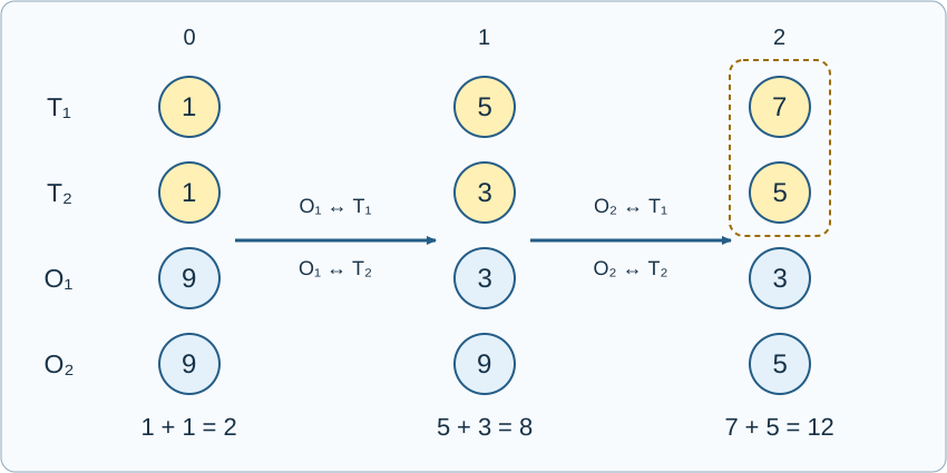
Sort everyone by nondecreasing wealth, labeling targets \(T\) and outsiders \(O\) . Whenever adjacent labels are \(TO\) , average those two values and exchange their positions in the sorted list. Their values are equal afterward, so the list remains sorted. Continue until all \(O\) labels precede all \(T\) labels. Let \(\Phi\) be the resulting target sum.
The choice of operations does not affect the result. Each operation removes one label inversion. Two simultaneously available \(TO\) pairs cannot overlap, so their operations commute. Induction on the number of inversions gives the same final wealth vector for every execution order.
Each operation does not decrease target wealth. The target in a pair is no richer than the outsider. Thus \(\Phi\) is at least the current target sum, and it is reachable in finitely many edits.
No pairwise average increases \(\Phi\) . Fix the initial wealth ordering. The operations are then a fixed sequence of adjacent averaging matrices, making \(\Phi\) linear in the initial coordinates. At the end, the target-sum coefficients in sorted order are
Propagating these coefficients backward averages adjacent coefficients at each step, preserving their nondecreasing order. A richer initial coordinate therefore has a coefficient at least as large as a poorer coordinate.
Now continuously bring any two values \(x<y\) toward their mean. On a segment with fixed ordering, their coefficients satisfy \(c_x\le c_y\) . Transferring \(\delta\) to the poorer coordinate changes the potential by
The function is continuous when the ordering changes. Exchanging equal-valued residents of the same type has no effect. For different types, first perform the zero-change \(TO\) operation at equality to obtain the other ordering’s problem. There are finitely many ordering segments, so averaging the pair cannot increase \(\Phi\) .
Averaging a larger group also cannot increase \(\Phi\) . Repeated pairwise averages within that group approach its common mean. Continuity extends the bound to this limit. The limit is used only to prove an upper bound; the strategy attaining it remains finite.
After any edits, the target sum is at most the current \(\Phi\) , which is at most its initial value. The adjacent strategy attains that initial value, proving optimality. Related discrete averaging models are studied by Hay, Schiff, and Fisch. The proof here establishes the specific potential directly, without enumerating extreme points of the general model.
A Grid for the Optimal Strategy
Initially every target has wealth \(a\) . Outsiders with wealth at most \(a\) already precede the targets and need no operation. Sort the remaining \(r\) outsiders as \(v_1\le\cdots\le v_r\) .
Process outsiders in that order. Each averages with targets from currently richest to poorest and is never used again afterward. If \(x_{i,j}\) is the common value after outsider \(j\) averages with target \(i\) , then
The answer is \(\sum_{i=1}^{k}x_{i,r}\) . This recurrence is useful for small-instance checks, but the population can approach \(10^{12}\) , so it cannot be expanded in the full solution.
One Outsider’s Contribution
Subtract \(a\) from every value, making all target initial values zero. If an outsider has \(t\) later outsiders, the coefficient of its excess wealth \(v-a\) in the final target sum is
This counts grid paths from that column’s top boundary to row \(i\) of the last column. There are \(\binom{t+i-1}{i-1}\) paths, each containing \(i+t\) halvings.
Define the coefficient tail \(T(r)=\sum_{t=r}^{\infty}c_t\) . Reversing the summation order gives
To prove the identity, fix \(i\) . The term \(\binom{t+i-1}{i-1}/2^{t+i}\) is the probability that exactly \(t\) tails precede the \(i\)-th head in fair coin flips. Having at least \(r\) tails is equivalent to having \(j<i\) heads before the \(r\)-th tail. Its tail probability is therefore \(\sum_{j=0}^{i-1}\binom{r+j-1}{j}/2^{r+j}\) . Summing over \(i=1,\ldots,k\) counts each \(j\) exactly \(k-j\) times.
Processing an Entire Household
Scan households in decreasing initial per-capita wealth, keeping only those richer than \(a\) . Suppose \(r\) residents have already been scanned and the current household contains \(p\) residents of mean wealth \(v\) . Its combined contribution is
Add these contributions to \(m_1\) . Equal-mean households can appear in any order because their coefficient differences telescope.
Evaluate each finite sum for \(T(r)\) in \(O(k)\) operations using
Precompute modular inverses for \(1,\ldots,M\) and powers \(2^{-p}\) , where \(M=\max_i p_i\) . Update the running \(2^{-r}\) by multiplying it by \(2^{-p}\) . Compare initial means by integer cross-products, never by their residues.
The population count \(r\) may exceed \(P\) . The recurrence is still valid: it only divides by \(1,\ldots,k-1\) , all invertible. Do not replace it with factorial inverses involving \(r!\) . Denominators of the optimum use only initial household sizes and powers of two, hence are coprime to \(P\) . Use 64-bit integers for population sums and mean cross-products. Products of two residues also fit signed 64-bit integers.
Complexity, Alternatives, and Verification
Time is \(O(n\log n+nk+M)\) and space is \(O(n+M+k)\) . The reference stores inverse and power tables to reduce work per household.
The forward method maintains the \(k\) target values and batches equal outsiders using a finite binomial expansion of a lower-triangular matrix. It uses \(O(n+k)\) space but needs \(O(k^2+\log P+\log M)\) time per household. Full measurements and pass status for both methods are in the benchmark record. Recalibrate on other platforms.
Small inputs use an exact Fraction grid. Large grouped inputs use the literal one-person averaging matrix and generic matrix exponentiation. Two general full-size inputs are cross-checked between backward tails and forward convolution, supported by the proof; they are not independently exhaustively solved. Additional checks cover arbitrary subset averages, populations crossing the modulus, and invalid inputs and outputs. See reproduction instructions.